VEHICLE INTELLIGENCE & TRANSPORTATION ANALYSIS LABORATORY   University of California, Santa Barbara

Positional Error

Larger image

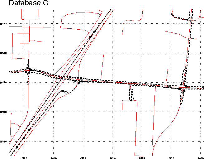
The red base map lines in this illustration are from vendor Knopf Engineering (Visalia CA), which claims an accuracy of about 0.6 metres, 55% of the time.  Driving eastbound and westbound down a major artery (horizontal line), the vehicle track straddles the centerline, as it should.  When the vehicle takes U-turns on side streets, the correspondence between the vehicle path and database is striking.  On the freeway (oblique parallel lines left of center) the vehicle path runs almost exactly down the centerline of the northbound and southbound carriageways.  If all street network data were this accurate, interoperability problems would be minimal.

Larger image

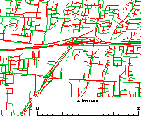
Using another reference database with the same drive path as above, significant positional errors are evident in the database.  Note the gross generalization of the ramp off the northbound carriageway of the freeway.  The grid interval is 200m.   This database is more typical of the commercial offerings currently on the market.  In fairness to these map database vendors, they serve a different market, and their price is more than an order of magnitude below that of the engineering-grade product above.

Disagreement — the Interoperability Problem

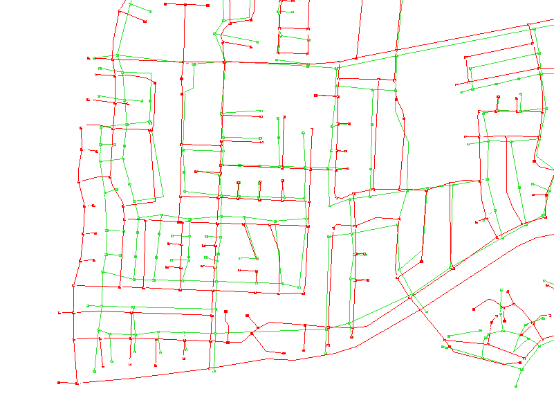
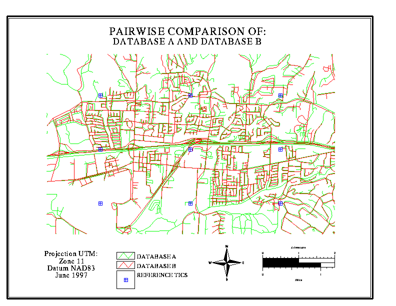
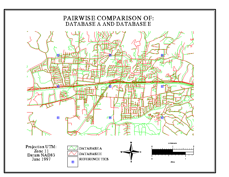
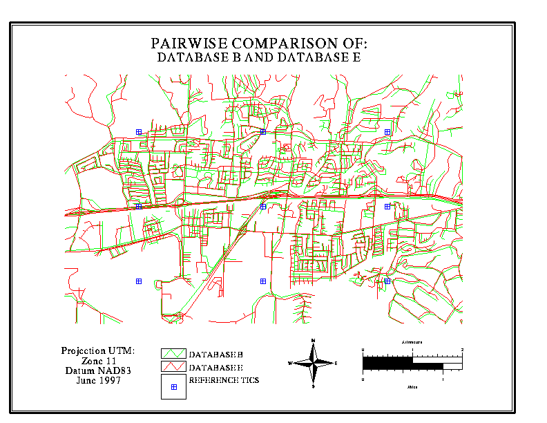
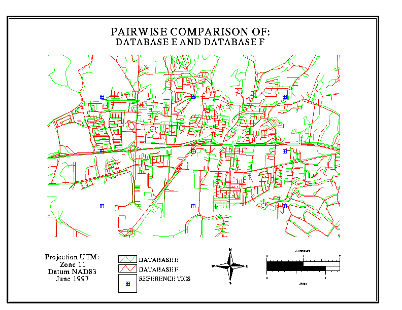
A graphic overlay is a simple yet dramatic way to illustrate the extent of disagreement, and the kinds of locations where disagreement is most likely to occur.  In the illustrations below, data bases for a section of Goleta (suburban Santa Barbara) are overlaid in pairs, one in red, the other in green.  Discordances of up to 100 metres are routinely observed in some neighbourhoods, while in other areas there is better agreement.  In the case of Map 5 (B vs F), one is known to be derived from the other; this is evident from the close agreement.
 

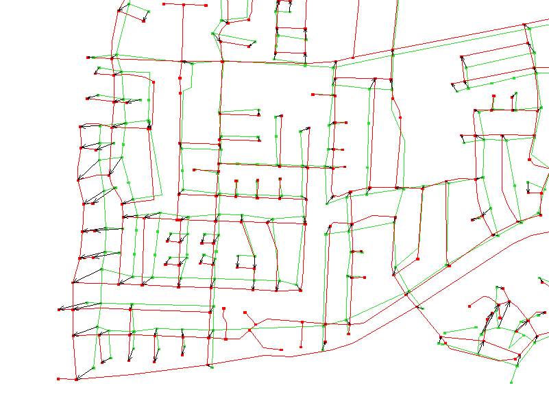
It is fair to argue that when two maps disagree, one or both contain error.  Examining a small section of one of the above maps closely, we find two types of error:   positional disagreement error of inclusion/exclusion: streets that appear in one data base and not the other These are the visible errors that are immediately evident from the overlay maps.  In addition there are disagreements on the spellings of street names and aliases, prefixes and suffixes, address ranges, link connectivities and attributes such as the number of lanes.

Origins of Disagreement

• Lack of standard control procedures in surveying — engineering plans for road construction are often laid out with reference to a local ground control station, but there is no immediate need from an engineering viewpoint to tie those station coordinates into a wider civic, state or national coordinate system.  As a result, maps develop piecemeal, and the components are subsequently collaged with inevitable stretching and twisting.
• Scale requirements — data may be gathered from small scale (1:100,000) maps or aerial photography, for a general purpose survey; but those data are inappropriate for navigation or other applications that require large scale (1:25,000) scale surveys.

Measuring Disagreement

Positional disagreement can be studied by identifying a set of points in one data base, finding the corresponding points in the other data base, and measuring the vector or positional difference between the two points.  The easiest points of correspondence to study are intersections.  They can be automatically identified with reference to the names of the intersecting streets (the process is not error-proof — see our comments on the Cross-Streets Profile).  In the figures below, intersections have been identified automatically within a small neighborhood in Goleta, California.  The databases are in red and green, the vectors in black.    Databases only Larger image Databases with disagreement vectors Larger image Vector field Larger image If one database can be considered “true” (usually by virtue of having been surveyed at a larger scale), then the vectors are a measure of the distribution of error in the other database.

Modelling Error

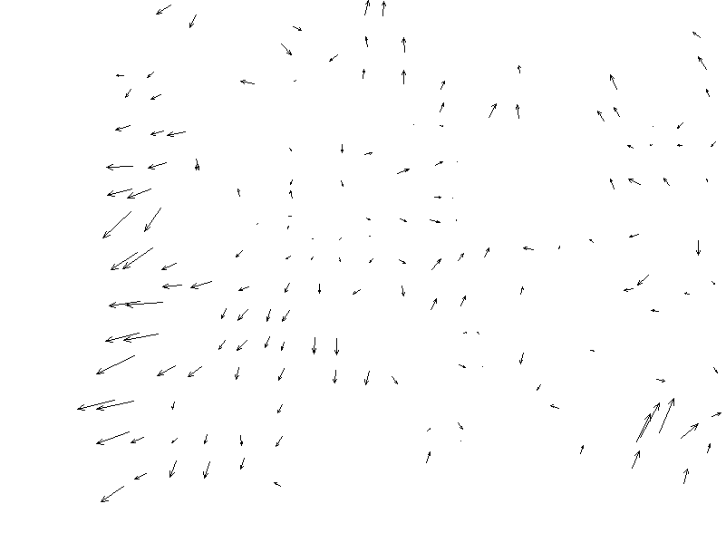
The set of black vectors may be considered a sample of a vector field, i.e. at every point on the map there is a local error, of which the yellow vectors represent a sample.  At VITAL we are trying to characterize error fields in different ways.  If the magnitude and direction of error is consistent in one portion of the map, it would suggest that that area was surveyed or digitized at the same time, by the same operator, with a constant error.  Once we have a satisfactory means of modelling error, we can consider the error at any point to be a function of two components: (a) systematic error as characterized by the field, and (b) random error at the point.  Error due to (a) can be corrected, leaving only random residual error.  Two of our technical reports (Church et al, 1998; Funk et al, 1998) describe our most recent efforts in error modeling.

Larger image